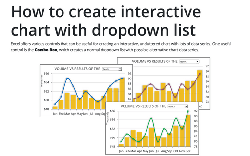
How to create interactive chart with dropdown list in Excel

See also interactive charts.

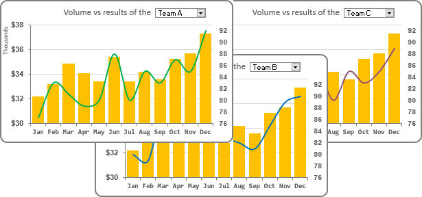
To create an interactive chart with a drop-down list, do the following:

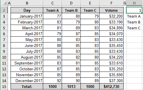
   1.   Add additional data to your spreadsheet for drop-down list values:

• Number as an index of the selected list item,
• All items in one column if you want to create a list from the column names (if you want to create a list of row names, this step isn't needed).

For example:

• Enter in the cell H2 the number 1,
• Column names in the range H3:H5 (see How to change columns to rows and vice versa):

   2.   Create data ranges, which will be used for the interactive chart:

   2.1.   On the Formulas tab, in the Defined Names group, click Define Name (see Creating and using named ranges for more details):

   2.2.   In the New Name dialog box:

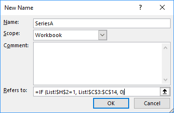
• In the Name field, enter the name of this new range, for example, SeriesA,
• In the Refers to field, enter this formula:

= IF (<condition>, <series data>, 0)

Where the condition is the option to show this data series.

In this example:

= IF ($H$2=1, $C$3:$C$14, 0):

   2.3.   Add the new data range for the other series.

In this example:

• Second data range:
  • Name: SeriesB,
  • Refers to: = IF ($H$2=2, $D$3:$D$14, 0),
• Third data range:
  • Name: SeriesC,
  • Refers to: = IF ($H$2=3, $E$3:$E$14, 0).

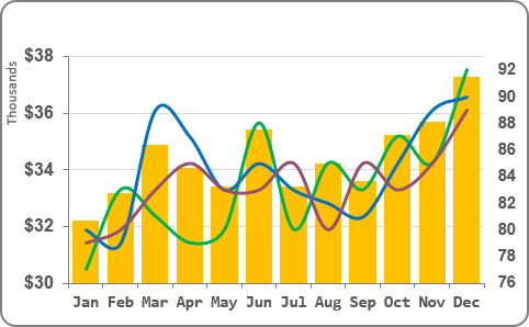
   3.   Create a chart that includes all data series:

   4.   Change the data series:

   4.1.   Do one of the following:

• Under Chart Tools, on the Design tab, in the Data group, choose Select Data:
  
• Right-click in the chart area and choose Select Data... in the popup menu:
  

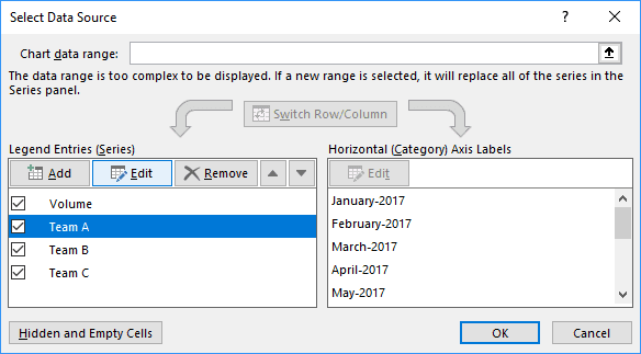
   4.2.   On the Select Data Source dialog box, for the Legend Entries (Series), select the first data series that you would like to show using the drop-down list and click the Edit button:

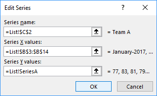
   4.3.   In the Edit Series dialog box, change Series name and Series Y values (or Series values) to the appropriate names:

   4.4.   Repeat the previous steps for all other data series that you will show using the drop-down list.

   5.   Add the drop-down list to the chart:

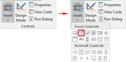
   5.1.   On the Developer tab (see Show the Developer tab), in the Controls group, click the Insert drop-down list and then choose Combo Box:

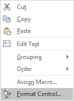
   5.2.   Right-click on the drop-down list and choose Format Control... in the popup menu:

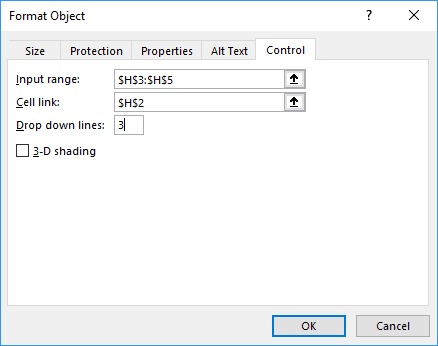
   5.3.   In the Format Control dialog box, on the Control tab:

• In the Input range field, select the range of item names (in this example, H3:H5),
• In the Cell link field, select the cell with the index of the selected item (in this example, H2),
• In the Drop down lines field, type the number of items in the list:

Make any other adjustments to get the look you desire.

Note: To show data series, Excel will use the colors from the theme by default. To use your colors for checked data series, create a new theme with custom colors. For example:

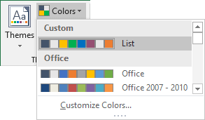
See How to change the default colors that Excel uses for chart series for more details.

See also this tip in French: Comment créer un graphique interactif avec une liste déroulante dans Excel.