How to draw flowchart and swimlane flow chart in Excel
Flowcharts often have specific names, such as process map, functional flowchart, process diagram, business plan, workflow diagram, functional block diagram, business process modeling, business process model and notation (BPMN), workflow diagram ( PFD), etc.:
Many different SmartArt templates predefined in MS Excel can be used to illustrate the process, including visually appealing templates with pictures.
However, if you want to use different shapes and a complex topology, it is better to create your own flowchart.
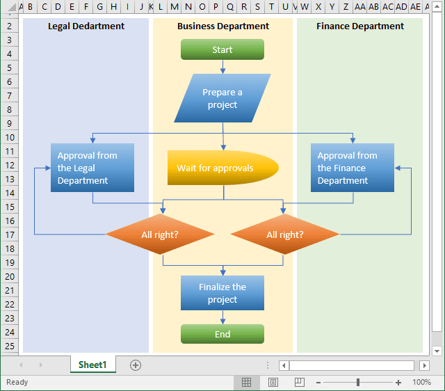
One of the most used flowchart types is a swimlane flowchart. A swimlane chart (also known as a cross-functional diagram or a cross-channel flow) describes which actions or steps are performed by which agents (persons, departments, entities) in a process. The main feature of this type of flowchart is that the elements in the flowchart are placed and mapped to each other on the lanes corresponding to different process agents:
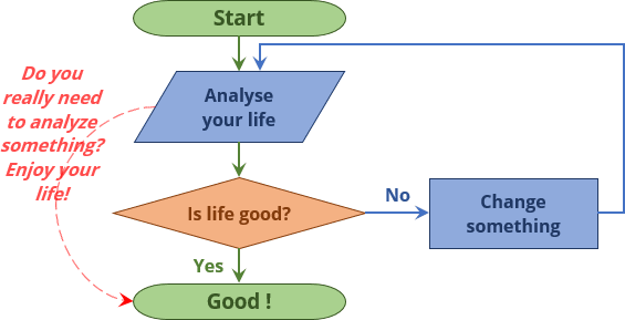
No wonder that building blocks and rules of flow charts were standardized by the American National Standards Institute (ANSI) and International Organization for Standards (ISO) more than 50 years ago. The current standard defines the drawing direction from top to bottom and left to right and specific symbols for different types of entities, actions, etc. E.g.:
| Rectangle with round corners marks for starting and terminating states | |
 |
Box with straight corners represents the process stages |
 |
Parallelogram illustrates data input/output |
 |
Diamond marks conditional branching |
| Arrow shows the process flow |
You can find all these and other useful visual elements in the Shapes dropdown list of the Insert tab in Excel. See more about different shapes for flowchart steps and lines.
To create a flowchart in Excel, follow the next steps (we recommend seeing how to change the width of gridlines in Excel and easily organize shapes in Excel that simplify the drawing):
1. On the Insert tab, in the Illustrations group, click the Shapes button:
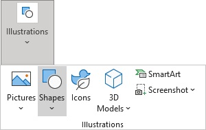
2. On the Shapes list, in the Flowchart group, choose the item that you prefer:
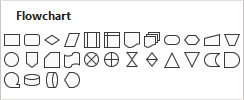
See the full list of the Flowchart shapes with their description.
3. To add text in the selected shape, just double-click on it and enter the text.
4. To connect shapes, on the Insert tab, in the Illustrations group, click the Shapes button, then select one of the connectors from the Lines group:

See the full list of the Flowline shapes with their description.
Almost all shapes have connection points, the special anchors to which connectors can be attached (or glued). The connection points are displayed as small gray circles:

Note: Connection points only become visible when you select any connector and try to connect one shape to another. Connection points become visible on hovering over the selected line next to the shape.
The connection between a shape and a connector is established, and the gray circle of the connector turns green. The connection attaches to the shape, so it will move with the shape when you move one of the attached shapes. Make sure the start and end of the connection are always shown in green:
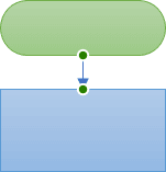
Otherwise, when moving shapes, unconnected points hang loosely:
- Attached is the arrow connecting both shapes:
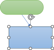
- Loose is the arrow connecting only to one connection point:
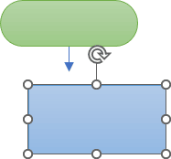
Note: Word, Excel, and Powerpoint are not specialized flowchart applications like Visio, so they do not have a tool for creating dynamic connections (a dynamic connection is a connection where the connector flows around the shape as it moves). Sometimes you have to reconnect or reroute connections after moving shapes.
5. Add as many shapes as you need and connect them using shapes from the Shapes list.
For customizations of shapes and connectors, see:
- How to change the format for diagram shapes in Excel,
- How to change flowchart shapes in Excel,
- How to change connector type for the flowchart.
6. If you need to create a swimlane, you can add some blocks to define the areas of responsibility.
To add blocks to the flowchart, follow the next steps:
6.1. On the Insert tab, in the Text group, click the Text Box button:
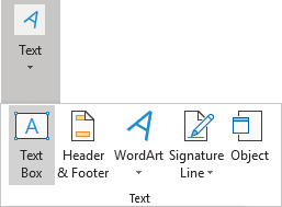
Note: Instead of the text box, you can use the simple rectangular shape from the Rectangles group of the Shapes list:

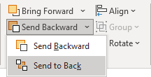
6.2. Position the new area (text box or shape) behind the flowchart by doing the following:
6.2.1. Select the text box or shape you want to put behind the flowchart.
6.2.2. On the Shape Format tab, in the Arrange group, click the Send Backward button, then choose Send to Back:
6.3. Double-click on the text box to add the text you need, such as a person or department name.
By default, the text is placed in the top left corner of the text box. To position it on the top-center, select the text, then do one of the following:
- Right-click the text box, then select Format Shape... in the popup menu:
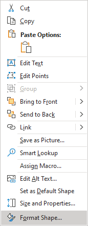
On the Format Shape pane, do one of the following:
- On the Text Options tab, in the Textbox group, in the Text Box section,
choose Top Centered from the Vertical alignment dropdown list:
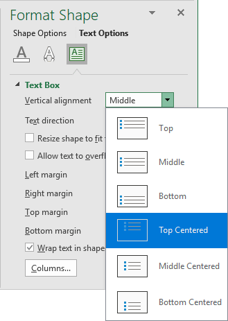
- On the Shape Options tab, in the Size & Properties group, in the
Text Box section, choose Top Centered from the Vertical alignment
dropdown list:
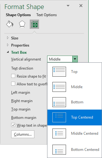
Note: Choose the Middle option if you position lanes vertically.
- On the Text Options tab, in the Textbox group, in the Text Box section,
choose Top Centered from the Vertical alignment dropdown list:
- On the Home tab, in the Alignment group, select both Top Align and
Center buttons:

Note: Select the Middle and Left buttons if you position lanes vertically.
6.4. Format the text box (shape) as you prefer by doing the following:
- Right-click the text box, then select Format Shape... in the popup menu. On the Format
Shape pane, on the Shape Options tab, in the Fill & Line group:
- In the Fill section, select select the option you prefer (see more about filling and outline in Microsoft),
- In the Line section, select the option you prefer:
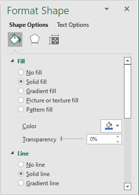
- On the Shape Format tab, in the Shape Styles group:
- Click the Shape Fill button, then select the filling option you prefer:
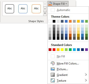
- Click the Shape Outline button, then select the outline option you prefer:
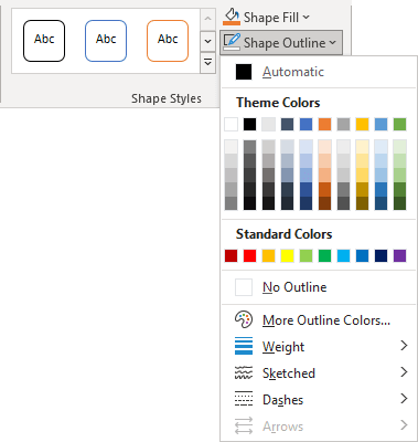
- Click the Shape Fill button, then select the filling option you prefer:
Note: You can use one workaround in Excel - just fill spreadsheet cells with the desired color, turn off the gridlines, and change their dimensions to create the needed areas (see an example above).
See also this tip in French: Comment créer un organigramme des opérations dans Excel.
