Glossy Gantt chart with a vertical line

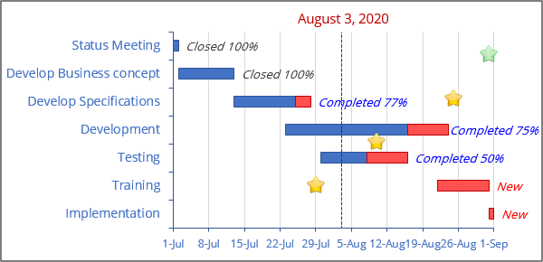
To add a vertical line with the current date to the existing Gantt chart, do the following:

Add a new data

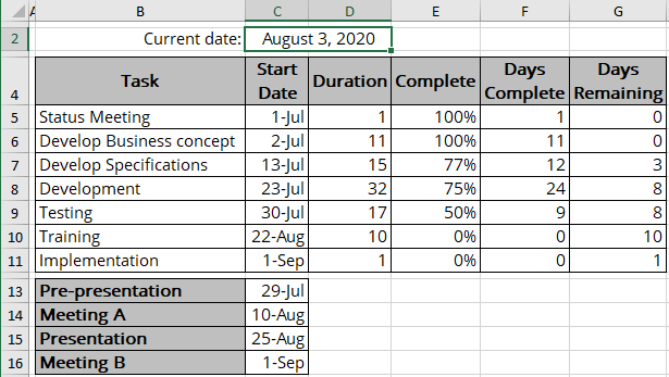
   1.   Add the current date to your spreadsheet.

You can use the TODAY () function that returns the current date or just type some data. Don't forget to format the cell to see the correct data.

For example, cell $C$2:

Add the new data series to the chart

   2.   Do one of the following:

• Select the chart, then on the Chart Design tab, in the Data group, choose Select Data:
  
• Right-click on the chart area and choose Select Data... in the popup menu:
  

In the Select Data Source dialog box, click the Add button, then in the Edit Series dialog box:

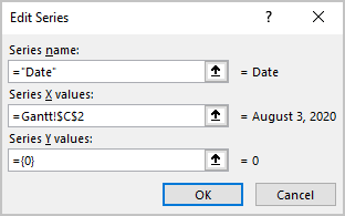
• If you add the vertical line to the chart with events (there is at least one scatter data series):
  • In the Series X values box - the cells with the date (in this example, $C$2),
  • In the Series Y values box - the constant value to see the new data point on the horizontal axis (for example, {0}):
  
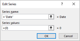
• If you add the vertical line to the simple Gantt chart or Progress Gantt chart (there are no scatter data series on the chart):
  

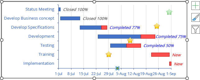
After clicking the OK button twice, Excel adds the new data to the chart:

Note: If you added a new data series to the Gantt chart without events, you need two additional steps:

   2.1.   Change the data series chart type:

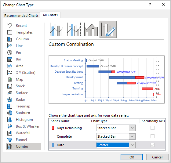
Right-click on any data series and choose Change Series Chart Type... in the popup menu:

In the Change Chart Type dialog box, for the new data series, choose the Scatter type (the Secondary Axis checkbox is selected automatically):

   2.2.   Correct the data series:

Open the Select Data Source dialog box, select the added data series and click the Edit button.

In the Edit Series dialog box, in the Series X values box, select the cell with the date (in this example, $C$2):

After clicking the OK button twice, Excel adds the new data to the chart:

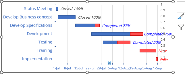
Add the vertical line

   3.   Select the new data, then do one of the following:

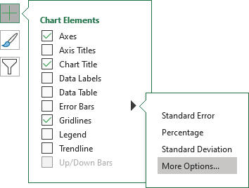
• Click on the Chart Elements button, select the Error Bars list, then choose More Options...:
  
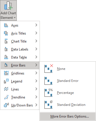
• On the Chart Design tab, in the Chart Layouts group, click the Add Chart Element dropdown list:
  

  In the Add Chart Element dropdown list, choose the Error Bars list, then click More Error Bars Options...:

  

See more about other options in Adding Error bars.

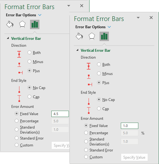
 - Customize the Y Error Bars: on the Format Error Bars pane, type parameters of the vertical line:

 - Remove the X Error Bars by selecting this chart element and clicking the Delete key. See how to select different chart elements quickly.

Correct and hide the secondary vertical axis

   4.   Do the following:

   4.1.   Right-click on the secondary vertical axis and select Format Axis... in the popup menu (or double-click the axis):

   4.2.   On the Format Axis pane, on the Axis Options tab:

• In the Axis Options section, correct the value in the Maximum field:
  • 4.5 for the Gantt chart with events,
  • 1.0 for the Gantt chart without events:
  
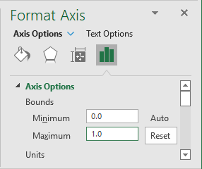
• In the Labels section, from the Label Position list, choose None:

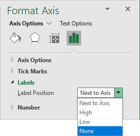
   5.   Make the new data series invisible. See also How to add a vertical line to the chart.

You can then make any other adjustments to get the look you desire.

See also this tip in French: Comment créer un diagramme de Gantt brillant avec une ligne verticale.