How to create a dependent drop-down list

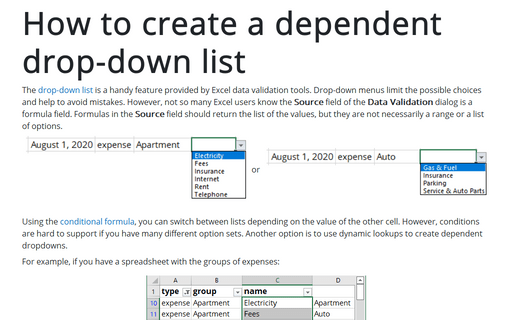
Using the conditional formula, you can switch between lists depending on the value of the other cell. However, conditions are hard to support if you have many different option sets. Another option is to use dynamic lookups to create dependent dropdowns.

For example, if you have a spreadsheet with the groups of expenses:

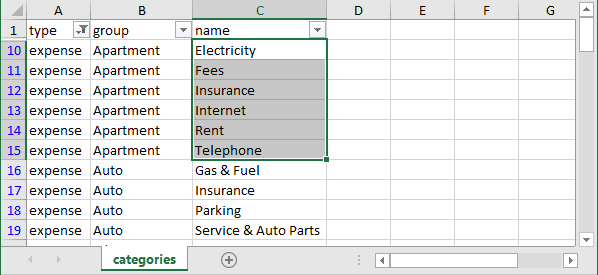
In this spreadsheet, there are more than ten different groups of expenses, and each group contains different kinds of expenses. To create dependent lists of expenses, do the following:

   1.   Create a named range (see Creating and using named ranges), for each group of expenses, for example:

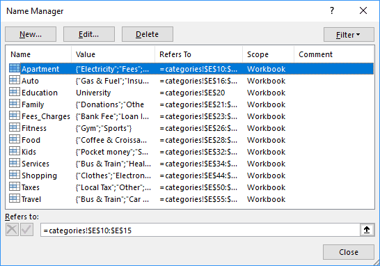
Note: To simplify future customizations, the name of the expenses group for as a range name. If your group name has two or more words, use symbol "_" (as "Fees & Charges").

   2.   Create the drop-down list for groups (see Creating a drop-down list in a cell):

   2.1.   On the Data tab, in the Data Tools group, click Data Validation:

   2.2.   In the Data Validation dialog box, on the Settings tab:

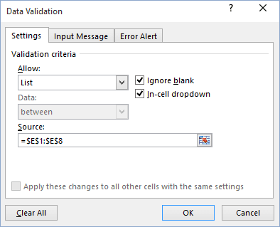
• In the Allow drop-down list, select the List item.
• In the Source box, specify the range that contains the items.
• Make sure to check the In-Cell Dropdown option.

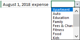
You will see the drop-down list:

   3.   Create the dependent drop-down list for selecting expense types:

   3.1.   On the Data tab, in the Data Tools group, click Data Validation.

   3.2.   In the Data Validation dialog box, on the Settings tab:

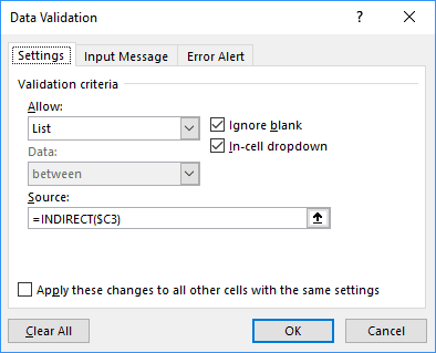
• In the Allow drop-down list, select the List item.
• In the Source box, specify the range:

  = INDIRECT (<cell_with_name_of_range>).

  Note: If it is necessary to make any changes for the name, use the text manipulation formulas, for example:

  = INDIRECT (SUBSTITUTE (<cell_with_name_of_range>, <old_text>, <new_text>))

  where

  • SUBSTITUTE converts Fees & Charges to the proper range name Fees_Charges
  • INDIRECT returns named range values for the specified range name.

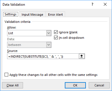
• Make sure to check the In-Cell Dropdown option.

   4.   Click OK:

See also this tip in French: Comment créer une liste déroulante dépendante.