Show chart data in hidden cells

See also how Excel displays the empty data on the chart.

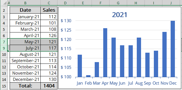
For example, there is some hidden data in the table:

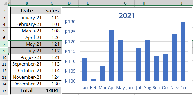
If you want to see hidden data in the chart, do the following:

   1.   Select the chart data by doing one of the following:

• On the Chart Design tab, in the Data group, choose Select Data:
  
• Right-click on the chart plot area and choose Select Data... in the popup menu:
  

   2.   In the Select Data Source dialog box, click the Hidden and Empty Cells button:

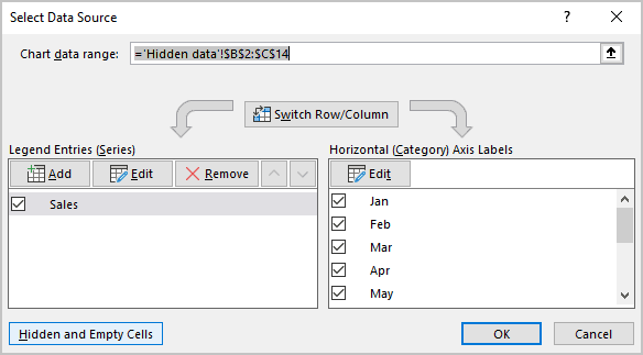
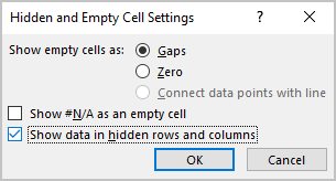
   3.   In the Hidden and Empty Cell Settings dialog box, check the Show data in hidden rows and columns checkbox:

Excel will show all hidden data on your chart:

See also this tip in French: Afficher les données du graphique dans les cellules masquées.