Show chart data for empty cells

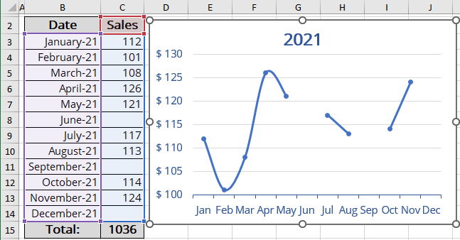
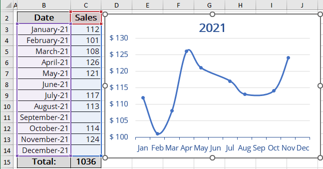
For example, there are some gaps or empty cells in the chart data table:

If you want to see average values in the chart, do the following:

   1.   Select the chart data by doing one of the following:

• On the Chart Design tab, in the Data group, choose Select Data:
  
• Right-click on the chart plot area and choose Select Data... in the popup menu:
  

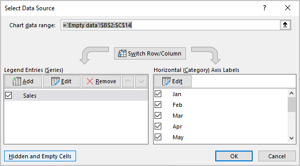
   2.   In the Select Data Source dialog box, click the Hidden and Empty Cells button:

   3.   In the Hidden and Empty Cell Settings dialog box, in the Show empty cell as option groups, select the Connect data points with line option:

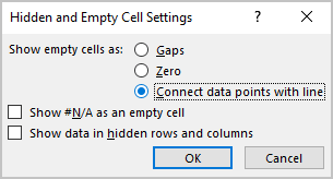
Note: This option is only available if there is some empty data or data with #N/A errors in the source data. To display data with #N/A errors in the same way as the empty cells, select the Show #N/A as an empty cell checkbox.

Excel will calculate and display the interpolated data instead of the empty cells on your chart:

See also this tip in French: Afficher les données du graphique pour les cellules vides.