Unrealized Gain and Loss

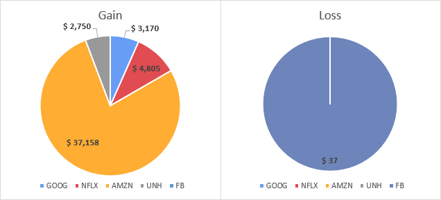
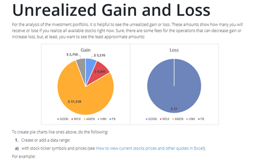
To create pie charts like ones above, do the following:

   1.   Create or add a data range:

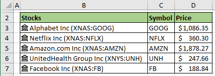
   a)   with stock ticker symbols and prices (see How to view current stocks prices and other quotes in Excel).

For example:

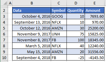
   b)   with transactions (if you have a fixed quantity, you can add them without an additional calculation).

For example:

   2.   Add new columns to calculate current value, Gain and Loss:

• Quantity (if you have fixed quantity, you can add them without additional calculation) using the following formula:

  = SUMIFS (Transactions[Quantity], Transactions[Symbol], "="&<symbol>)

  where:

  • SUMIFS is a function to sum cells that meet multiple criteria:

    SUMIFS (<the range to be summed>, <the first range to evaluate>, <the criteria for the first range>, [<the second range>], [<the criteria for the second range>], ...)

  • Transactions is a table from ppoint 1.b),
  • <symbol> is a stock symbol from column C.

  For the cell E4 this formula is:

  = SUMIFS (Transactions[Quantity], Transactions[Data], "="&C3):

  
• Value using the formula:

  = <price> * <quantity>

  For the cell F4 this formula is:

  = D4 * E4:

  

  Note: You can hide the price and quantity data and use the formula:

  = <stock>.Price * SUMIFS (Transactions[Quantity], Transactions[Symbol], "="&<symbol>)

  where, <stock>.Price is a reference to the Price field of the Stocks data type.

  For example:

  
• Gain:

  = IF ((<value> - <cost>) > 0, <value> - <cost>, 0)

  where:

  • <value> is a calculated amount from the previous step,
  • <cost> can be calculated like a <quantity> using the formula:

    = SUMIFS (Transactions[Amount], Transactions[Symbol], "="&<symbol>)

  For this example:

  
• Loss:

  = IF ((<cost> - <value>) > 0, <cost> - <value>, 0)

  For this example:

  

   3.   Select the data range to create a pie chart.

For this example, C3:C7 and E3:E7.

   4.   On the Insert tab, in the Charts group, click the Insert Pie or Doughnut Chart button:

Choose the Pie chart :

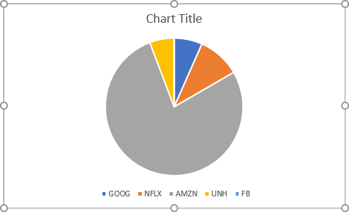
Make any other adjustments to get the look you need.