How to create drop-down list in Excel cell

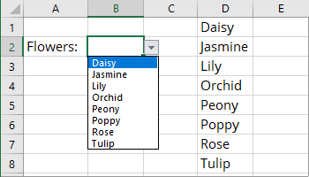
Create a drop-down list for the cell

To create a drop-down list for the cell, do the following:

   1.   Create a column or a row of the items in the active spreadsheet for the drop-down list. If the drop-down values list is short, you can skip this step.

   2.   Select the cell that needs a drop-down list for data validation (cell B2, in this example).

   3.   On the Data tab, in the Data Tools group, click Data Validation:

   4.   In the Data Validation dialog box:

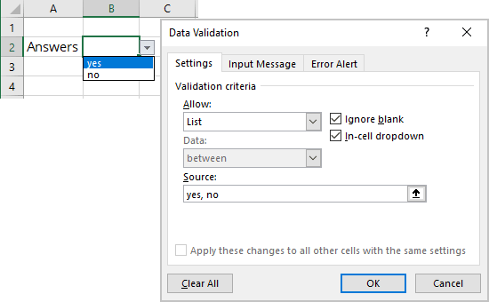
• On the Settings tab:
  
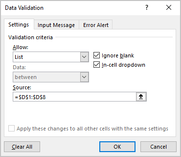
  • In the Allow drop-down list, select the List item.
  • In the Source box, specify the range that contains the drop-down list items (in this example, the range is D1:D8). If the number of drop-down values is small, type your list items (separated by commas) in the Source box in the Data Validation dialog box:
    

    Note: The list separator symbol can be also semicolon - it depends on the local customization. See how to change the list separator in Microsoft.

    For small data validation lists that are unlikely to change, a comma-separated (semicolon-separated) value drop-down list is the best option. You don't have to worry about finding a place to store the list values.

  • Check the In-cell dropdown option to show the drop-down list. Otherwise, Excel validates your data entry but does not show the drop-down button to select items from the list.
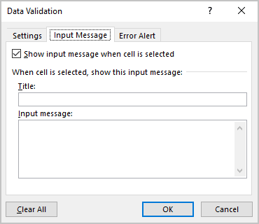
• On the Input Message tab:
  • To display a message pop-up that appears when the cell is clicked, select the Show input message when cell is selected check box, and type a title and message in the Title and Input message text fields (up to 225 characters).
  • Clear the checkbox if you don't want a message to appear:
  
• On the Error Alert tab:
  • To display an error message pop-up when someone enters something that's not in your list, select the Show error message after invalid data is entered check box, choose a pop-up style from the Style drop-down list, and type a title and message in the Title and Error message text fields:
    
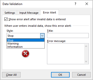
    • Choose the Information or Warning pop-up styles if you want to allow people to enter data that is not in the drop-down list.
    • Choose the Stop pop-up style if you want to prevent people from entering data that is not in the drop-down list.

    You can find pop-up examples in checking data entry for invalid entries.

    The title will be "Microsoft Excel", and the message will be "The value you entered is invalid. A user has restricted the values that can be entered in this cell" if you do not add a title or text.

  • Clear the check box if you don't want a message to appear.

   5.   Click OK.

Notes:

• In Excel 365, data validation lists support AutoComplete. To speed up data entry in large lists, start typing the target word in the drop-down menu cell. The AutoComplete algorithm compares the typed substring with the drop-down list items and shows you only the items that match. The more characters you type, the narrower the list you see; the more characters you remove, the more matches you see.
• You can hide the range of values used in the Source box or create it on the protected sheet that you can hide. To hide source values, right-click the source values column or row and select the Hide command from the context menu. If you later need to add new values to the cell drop-down list, select the adjacent columns or rows, and select the Unhide command from the context menu. You can also make the spreadsheet invisible to the Unhide command if the data for the cell drop-down list is on a separate spreadsheet.
• If you insert multiple drop-down menus on different sheets, using named ranges will make it much easier to identify and manage the drop-down menus.
• You can add the drop-down list to multiple cells by selecting the appropriate cells or copying/pasting the cell with a list.
• If you plan to share your workbook with users of Excel 2007 or earlier, ensure the list is on the same sheet as the drop-down list. Alternatively, you can use a named range.

Add/Remove items to the drop-down list

Excel automatically updates the Source fields in all cells that reference that range for data validation when you add a new row or column to the source range for the drop-down list. However, you will get a nasty surprise if you try to add a new element at the end. This problem is solved by automatically extended or dynamic drop-down lists.

To create a dynamic drop-down list, do the following:

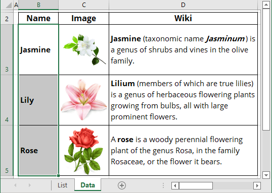
   1.   Enter the list of items in a range. For example:

   2.   Select the cell that will contain the drop-down list.

   3.   On the Data tab, in the Data Tools group, click Data Validation:

   4.   In the Data Validation dialog box, on the Settings tab:

• In the Allow drop-down list, select List.
• In the Source box, enter the following formula:

  = OFFSET (<first cell>, 0, 0, COUNTA (<column>), 1)

  For this example:

  = OFFSET (Data!$B$3, 0, 0, COUNTA (Data!$B:$B), 1)

  So, you ask Excel to return the data range of filled cells, starting from the <first cell> in the column (the function COUNTA () returns the number of cells that are not empty in a range).

  
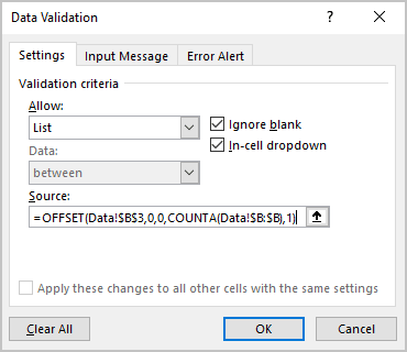
• Make sure that the In-cell dropdown option is checked. Otherwise, you will create a validation criteria without the ability to choose from a drop-down list.

   5.   Click OK.

Create the dependent drop-down list

Automatically extended or dynamic drop-down lists use custom formulas to reference source values. You can use conditional formulas with named ranges to create dependent drop-down lists with different validation lists for different parent values.

To create a dependent drop-down list, do the following:

   1.   Create named ranges for the dependent drop-down list (see Creating and using named ranges), for example:

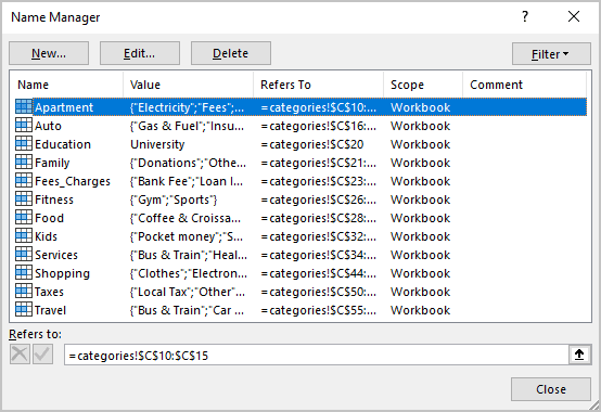
To simplify future customization, use the value of the parent dropdown list item as the name for the dependent named range.

   2.   Create the drop-down list for the parent cell (see how to create a simple dropdown list above).

You will see the drop-down list:

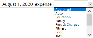
   3.   Create the dependent drop-down list:

   3.1.   On the Data tab, in the Data Tools group, click the Data Validation button.

   3.2.   In the Data Validation dialog box, on the Settings tab:

• In the Allow drop-down list, select the List item.
• In the Source box, specify the range:
  

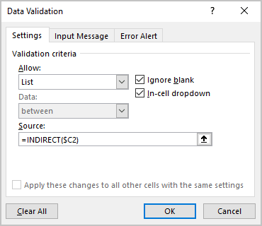
  = INDIRECT (<cell_with_name_of_range>).

  Note: If necessary to make any changes for the name, use the text manipulation formulas, for example:

  = INDIRECT (SUBSTITUTE (<cell_with_name_of_range>, <old_text>, <new_text>))

  where

  • SUBSTITUTE converts Fees & Charges to the proper range name Fees_Charges
  • INDIRECT returns named range values for the specified range name.
  
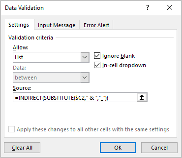
• Make sure to check the In-cell dropdown option.

   4.   Click OK.

You can create multiple drop-down lists with multiple criteria to build a hierarchy of drop-down entries.

Remove a drop-down list for the cell

   1.   Select the cell or range of cells with the drop-down list for data validation (cell B2, in this example).

   2.   On the Data tab, in the Data Tools group, click Data Validation:

   3.   In the Data Validation dialog box, on the Settings tab:

   4.   Click the Clear All button. Check the Apply these changes to all other cells with the same settings check box before clicking the Clear All button if you want to remove all other drop-down lists with similar settings.