How to show image linked to the list element
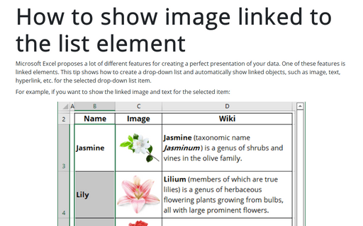
For example, if you want to show the linked image and text for the selected item:
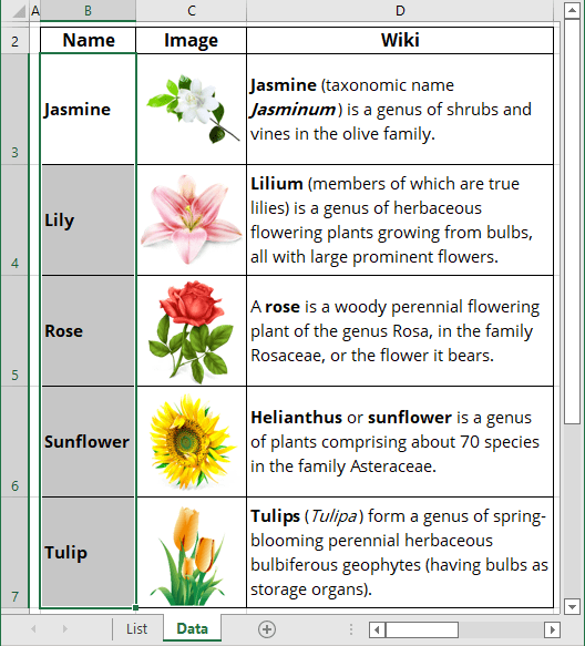
To create a drop-down list with linked images, do the following:
I. Create a drop-down list from your data (see Creating a drop-down list in a cell for more details):
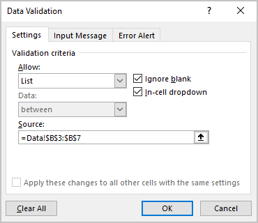
In this example the drop-down list was created in the List sheet:
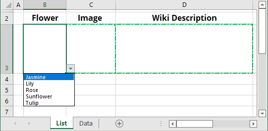
II. To show the linked picture of the selected item, do the following:
1. Create the name range of pictures:
1.1. On the Formulas tab, in the Defined Names group, click Define Name (see Creating and using named ranges for more details):

1.2. In the New Name dialog box:
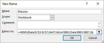
- In the Name field, enter the name of this new range, for example, Pictures,
- In the Refers to field, enter the formula:
= INDEX (<list of pictures>, MATCH (<selected item>, <list of items>, 0))
In this example:
= INDEX (Data!$C$3:$C$7, MATCH (List!$B$3, Data!$B$3:$B$7, 0))
2. Select any picture and copy it by doing one of the following:
- On the Home tab, in the Clipboard group, click the Copy button:

- Right-click in the selection and choose Copy in the popup menu,
- Click Ctrl+C.
3. Select the cell where you want to show the linked picture.
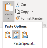
4. On the Home tab, in the Clipboard group, click on the Paste list and then choose one of the options:
- Keep Source Formatting:
- Picture:
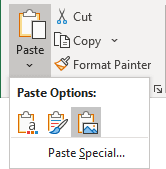
5. Select the pasted picture and in the Formula Bar type the name of your range (in this example, Pictures):
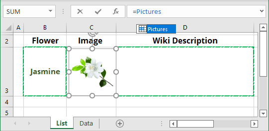
III. To show the linked text of the selected item, do the following:
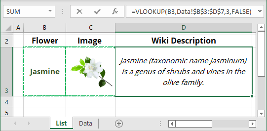
On the appropriate cell, where you want to see the linked text, enter the following formula:
= VLOOKUP (<selected item>, <data table>, <column to show>, <table option>)
where <table option> should be:
- TRUE, if items in your table are sorted,
- FALSE, if items should find an exact match.
In this example:
= VLOOKUP (B3, Data!$B$3:$D$7, 3, FALSE)
See also this tip in French: Comment afficher l’image liée à l’élément de liste.
