How to freeze columns and rows

To freeze row or column headings (or both), follow these steps:

   1.   On the worksheet, do one of the following:

• To lock rows, select the row below where you want the split to appear,
• To lock columns, select the column to the right of where you want the split to appear,
• To lock both rows and columns, click the cell below and to the right of where you want the split to appear:

   2.   On the View tab, in the Window group, click Freeze Panes:

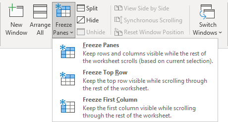
   3.   From the Freeze Panes drop-down list, choose the option that you want:

• The Freeze Panes option locks both rows and columns that are above and left the current cell.
• The Freeze Top Row option locks the first row in the sheet.
• The Freeze First Column option locks the first column in the sheet.

Excel inserts dark lines to indicate the frozen rows and columns. The frozen row and column remain visible while you scroll throughout the worksheet.

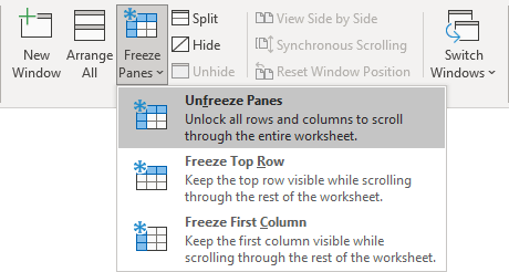
When you freeze panes, top row, or first column, the Freeze Panes option changes to Unfreeze Panes so that you can unlock frozen rows or columns:

See also this tip in French: Comment figer les colonnes et les lignes.