How to change default chart
To change this, follow the next steps:
1. Do one of the following:
- Select an existing chart, and then on the Chart Design tab, in the Type group,
click the Change Chart Type button:

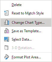
- Right-click on the chart area and select Change Chart Type... in the popup menu:

If you do not have an existing chart in your workbook, click the dialog box launcher on the Insert tab in the Charts group:

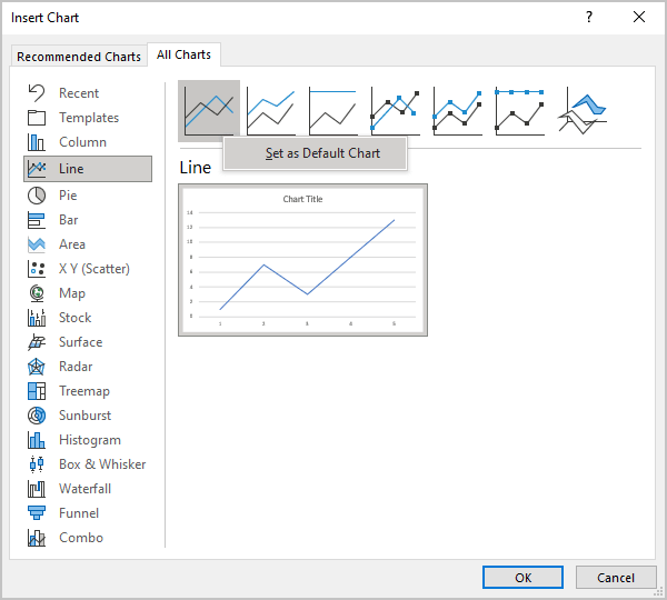
2. Select the chart subtype you want to set like a default chart.
3. Right-click on this chart to open the popup menu and select Set as Default Chart:

After you go through this procedure, you can press F11 or Alt+F1 to create the selected chart type instead of the column chart (see Using shortcut keys to create a chart). You can define a custom template as the default chart with custom colors, effects, and settings. See How to change the default colors that Excel uses for chart series for more details.
See also this tip in French: Comment changer le graphique par défaut.

