Competition chart with residual data
Excel 365 2013
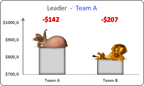
For some presentation of the competition will be more informative to see points that missed to achieve the Goal. This tip is about how to create a simple competition chart with residual data.
The Competition Chart Excel 2016

To create the chart like this one, do the following:

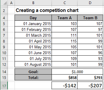
   1.   Add additional data to your chart to see the residual data (in this example, cells C17:D17).

   2.   Select all necessary data - in this example, C4:D4, C15:D15, C17:D17:
Data Competition Chart Excel 2016

   3.   On the Insert tab, in the Charts group, choose the Column button:

Bar Charts in Excel 2016

Choose the 100% Stacked Column 100% Stacked Column Charts in Excel 2016 chart.

   4.   Right-click on the second data series, then in the popup menu, select Add Data Labels and again Add Data Labels:

Add Data Label in Excel 2016

Make any other adjustments to get the look you desire. See more:

See also this tip in French: Créer un graphique de concurrence avec des données résiduelles.
Please, disable AdBlock and reload the page to continue

Today, 30% of our visitors use Ad-Block to block ads.We understand your pain with ads, but without ads, we won't be able to provide you with free content soon. If you need our content for work or study, please support our efforts and disable AdBlock for our site. As you will see, we have a lot of helpful information to share.

We use cookies to personalise content and ads, to provide social media features and to analyse our traffic. We also share information about your use of our site with our social media, advertising and analytics partners who may combine it with other information you’ve provided to them or they’ve collected from your use of their services.

Learn more