Conditional formatting for weekends

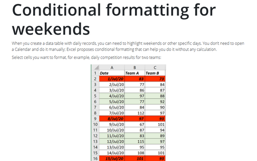
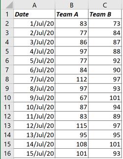
Select cells you want to format, for example, daily competition results for two teams:

To highlight weekends, do the following:

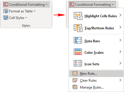
   1.   On the Home tab, in the Styles group, select the Conditional Formatting drop-down list, and then click New Rule...:

   2.   In the New Formatting Rule dialog box:

• In the Select a Rule Type list, select the Use a formula to determine which cells to format:
  
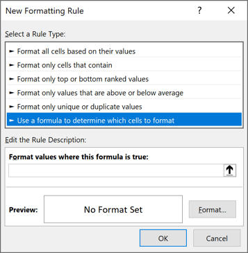
• In the Edit the Rule Description group:
  • In the Format values where this formula is true field enter the formula:

    = WEEKDAY (<date range>, 2) > 5:

    

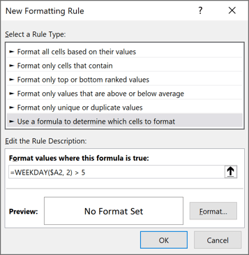
    The formula WEEKDAY returns a number between 1 and 7 that corresponds to a particular day of the week. With return_type = 2: 1 = Monday, 2 = Tuesday, 3 = Wednesday, 4 = Thursday, 5 = Friday, 6 = Saturday and 7 = Sunday.

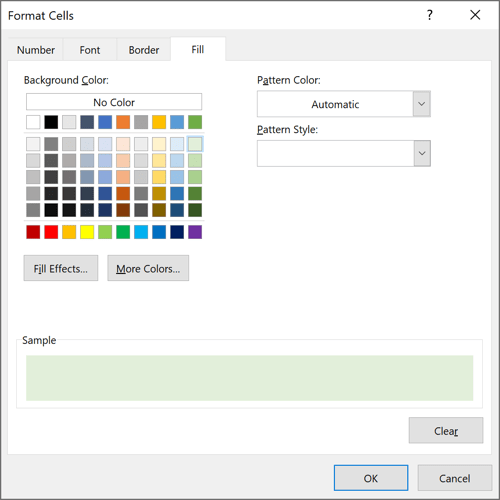
  • Click on the Format... button to select a format for these cells, for example, add background color:
    
• Click OK:

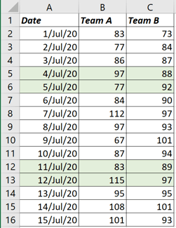
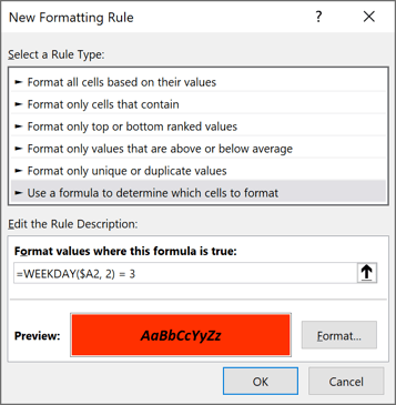
You can create several different formulas for the same cells. For example, to highlight Wednesdays in red as control days:

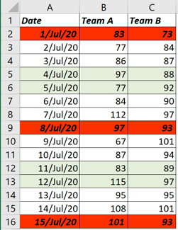
You will see the highlighted data without calculating weekdays:

See also this tip in French: Mise en forme conditionnelle pour les week-ends.