How to count cells by criteria

To count cells by criteria, do the following:

   1.   Select the cell where want Excel to return the number of cell by criteria.

   2.   Do one of the following to open the Insert Function dialog box:

• Select Insert -> Function...
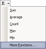
• Click the Sum button in the Standard toolbar and then select More Functions...:
  
• Click the Insert Function button in the left of the edit bar:
  

   3.   In the Insert Function dialog box full following fields:

• select Statistical in the Or select a category listbox
• select COUNTIF in the Select a function list

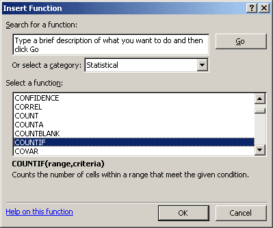
Then press OK.

   4.   In the Function Arguments dialog box, fill following fields:

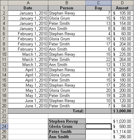
• The Range field determines the range of cells Excel will look to perform the count in. In this example the cell range is D2:D20.
• The Criteria is a conditional statement that is similar to the conditional statement in the IF statement.

   5.   Press OK.

Note: You can enter this formula using keyboard, for this example:

= COUNTIF (D2:D20, ">100")

If you want to use COUNTIF on a selection of cells (not necessarily one solid range), summing multiple COUNTIFs:

= SUM (COUNTIF (D3, ">100"), COUNTIF (D7, ">100"), COUNTIF (D14, ">100"), COUNTIF (D17, ">100"))

Note:

• You can use the wildcard characters, question mark (?) and asterisk (*), in criteria. A question mark matches any single character; an asterisk matches any sequence of characters. If you want to find an actual question mark or asterisk, type a tilde (~) before the character.
• Microsoft Excel provides additional functions that can be used to analyze your data based on a condition.
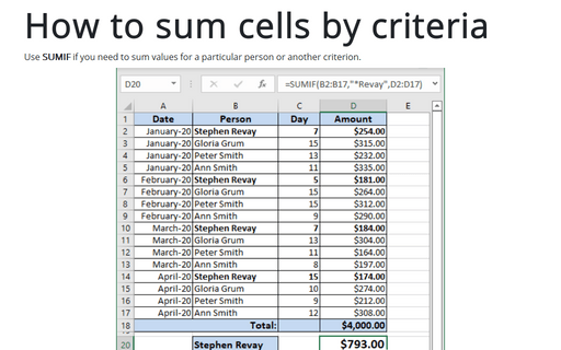
  • To calculate a sum based on a string of text or a number within a range, use the SUMIF worksheet function (see How to sum cells by criteria for more details).
  • To have a formula return one of two values based on a condition, such as a sales bonus based on a specified sales amount, use the IF worksheet function.
  • To count cells that are empty or not empty, use the COUNTA and COUNTBLANK functions.