Excel 3-D Pie charts
If you want to create a pie chart that shows your company (in this example - Company B) in the greatest positive light:
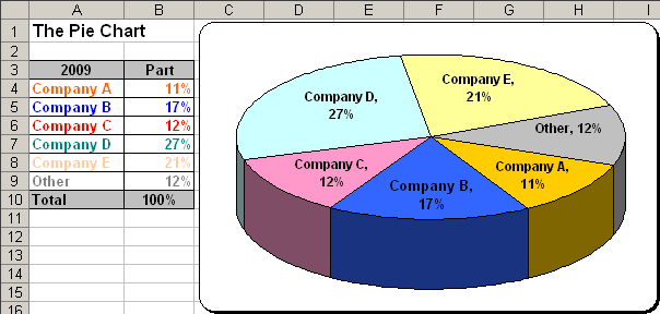
Do the following:
1. Select the data range (in this example A4:B9).
2. Select Insert -> Chart... to open the Chart Wizard dialog box:
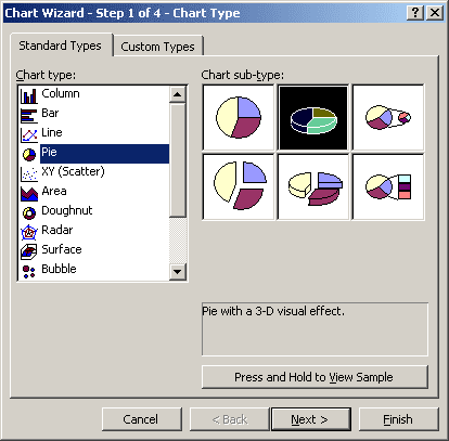
Choose the Pie type, the Pie with a 3-D visual effect sub-type and then click Next >.
3. In the Step 2 of Chart Wizard check the data and click the Next > button.
4. In the Step 3 of Chart Wizard, hide the legend in the Legend tab, in the Data Labels tab, choose the Category name and Value checkboxes and then click Next >.
5. In the Step 4 of Chart Wizard, click the Finish button.
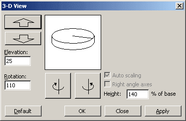
6. Right-click in the chart area. In the popup menu select 3-D View...
7. In the 3-D View dialog box:
- In Elevation type a number between 10 and 80. The default setting is 10 degrees.
- In Rotation choose most suitable values of the chart orientation.
- If you want to change the height of your chart, change the value in Height (% of base).
You can then make any other adjustments to get the look you desire.
