How to hide points on the chart axis
Excel
2013
Sometimes you need to omit some points of the chart axis, e.g., the zero point. This tip will show you how
to hide certain points on the chart axis using custom label format.
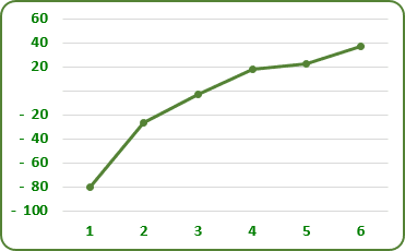
To hide some points in the Excel 2013 chart axis, do the following:
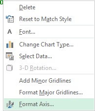
1. Right-click in the axis and choose Format Axis... in the popup menu:
2. On the Format Axis task pane, in the Number group, select Custom category and then change the field Format Code:
# ###;- # ###;;
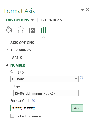
The first applies to positive values, the second to negative values, and the third to zero (for more details see Conditional formatting of chart axes).
3. Click the Add button.
