How to change default chart

To change this, follow next steps:

   1.   Select an existing chart and then on the Design tab, in the Type group, click the Change Chart Type button:

If you do not have an existing chart in your workbook, click the dialog box launcher on the Insert tab, in the Charts group:

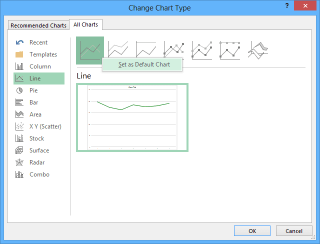
   2.   Select the chart subtype that you want to set like a default chart.

   3.   Right-click on this chart to open popup menu and select Set as Default Chart:

After you go through this procedure, you can press F11 or Alt+F1 to create the selected chart type instead of the column chart (see Using Shortcut keys to create a Chart). You can define a custom template as the default chart with custom colors, effects, and settings. For more details, see How to change the default colors that excel uses for chart series.