Glossy Gantt chart with a vertical line

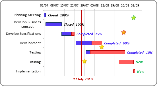
To add a vertical line in the current date, do the following:

   1.   Add the current date into your worksheet, select this cell, for example D1:

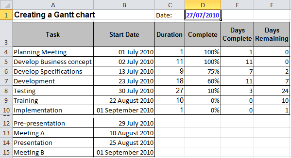
   2.   Do one of the following to add new data series with cell D1:

   1)   Add this cell to the events series (see Progress Gantt chart with events):

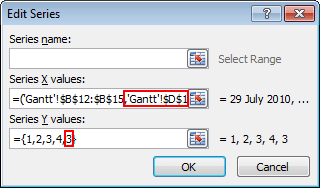
   2)   Add new data series with data cell D1:

• Do one of the following:
  • On the Design tab, in the Data group, choose Select Data:
    
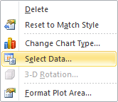
  • Right-click in the chart area and choose Select Data... in the popup menu:
    
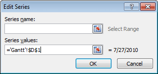
• In the Select Data Source dialog box, click the Add button and in the Edit Series dialog box, in the Series values box, select $D$1:
  
• Right-click in the new data series and choose Change Series Chart Type... in the popup menu. In the Change Chart Type dialog box, choose the Scatter with only Markers type
• Right-click in the chart area and choose Select Data... in the popup menu
• In the Select Data Source dialog box, select the new data series and click Edit
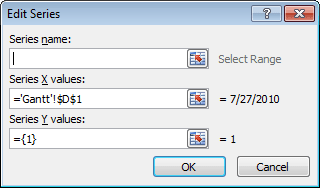
• In the Edit Series dialog box, correct data:
  • In the Series X values box - the cells with dates ($D$1)
  • In the Series Y values box - constant values (for example, {1}):
  
• Click OK twice
• Change the secondary axis parameters, and then remove it

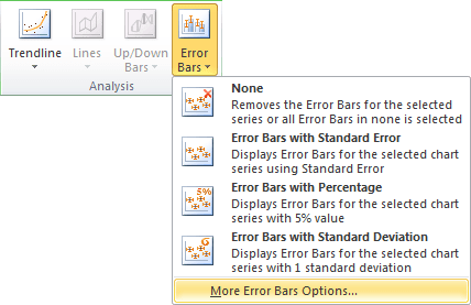
   3.   Select new date series, under Chart Tools, on the Layout tab, in the Analysis group, choose the Error Bars and then select More Error Bars Options...:

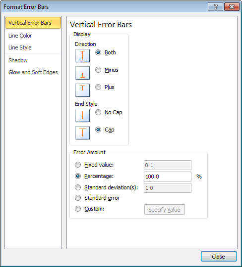
In the Format Error Bars dialog box, type parameters of the vertical line:

   4.   Make the new data series invisible.

You can then make any other adjustments to get the look you desire.