Waterfall chart using Error bars
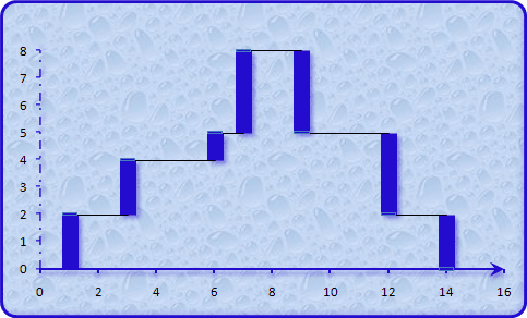
To create the waterfall chart using Error bars, do the following:
1. Add two columns with "X Errors" data and "Y Errors" data:
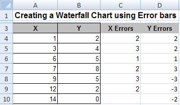
C4=A5-A4 and D4=B4, D5=B5-B4
2. Select the data range (in this example A4:B10).
3. On the Insert tab, in the Charts group, choose the Scatter button:

Choose Scatter with only Markers.
4. On the Layout tab, in the Analysis group, choose Error Bars list.

Excel propose several error bars, also you can use More Error Bars Options...:
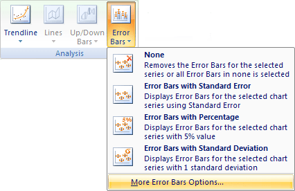
5. In the Format Error Bars dialog box:
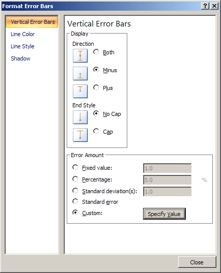
- In the Display Direction group, select Minus
- In the Display End Style group, select No Cap
- In the Error Amount group, near the Custom: click the Specify Value button.
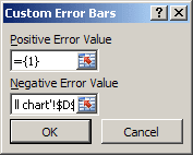
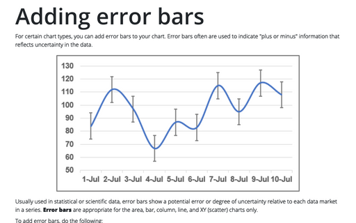
In the Custom Error Bars dialog box, choose the Y Errors data range (in this example D4:D10). See Adding error bars for more details about Error bars.
6. Right-click in one of the horizontal Error bars and choose Format Error Bars... in the popup menu:
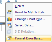
In the Format Error Bars dialog box, on the Horizontal Error Bars tab:
- In the Display Direction group, select Plus
- In the Display End Style group, select No Cap
- In the Error Amount group, near the Custom:, click the Specify Value button and then, in the Custom Error Bars dialog box, choose the X Errors data range (in this example C4:C9).
You can then make any other adjustments to get the look you desire.
