How to create a Scrolling chart

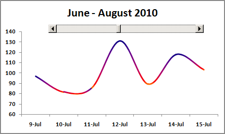
To create a chart like this one (sales data for the week for 3 months), do the following:

Step I: Create a chart

1. Select the data (in this example, A4:B95).
2. On the Insert ribbon, in the Charts group, choose Line:
   

   Choose the Line chart type, delete the legend.

Step II: Create an additional data

1. Enter 1 in any cell (for example, E1) - this number we will use for scrolling (scrolling cell).
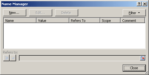
2. On the Formulas tab, in the Defined Names group, choose Name Manager:
   
3. In the Name Manager dialog box, click the New button:
   
4. In the New Name dialog box:
   
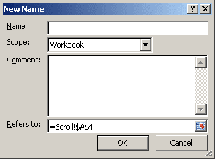
   • Type the name (for example, Dates) in the Name field.
   • In the Refers To field, enter:

     = OFFSET (Scroll!$A$4, Scroll!$E$1, 0, 7, 1).

     This says to start from cell A4 of the Scroll worksheet, move down the number of rows in cell E1, and then take a range that is 7 rows (one week) by first column.

5. Click OK to accept the name.
6. Add another name (for example, Sales). In the Refers To box, use:

   = OFFSET (Scroll!$A$4, Scroll!$E$1, 1, 7, 1).

   The only change is that in the third argument, you move right one column to grab data from column B.

7. Click the line series in the chart. Wait for the SERIES formula to appear in the formula bar. Edit the formula so that it looks like this:

   = SERIES (Scroll!$B$1, 'Charts-2007.xlsx'!Dates, 'Charts-2007.xlsx'!Sales, 1)

Test the chart. Enter a new number between 1 and the number of a last date (in this example, 92) in cell E1. The chart should change.

Step III: Add a scroll bar

On the Developer tab (if you don't have the Developer tab available in the ribbon, see Show the Developer tab), in the Controls group, click the Insert button and then choose the Scroll Bar icon:

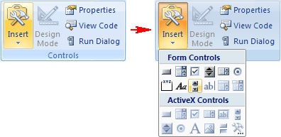
Note: You can also add the Scroll Bar control to the Quick Access Toolbar (see Adding commands to the Quick Access Toolbar):

Step IV: Customize the scroll bar

1. Right-click the scroll bar and choose Format Control... in the popup menu:
   
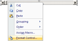
2. In the Format Control dialog box, on the Control tab:
   
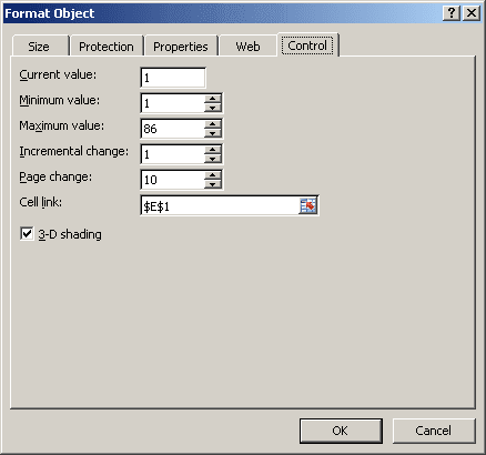
   • Change Minimum value to 1
   • Change Maximum value to your maximum value
   • Set Incremental Change to 1 (or if you want to 7, 10)
   • For Cell link, choose cell with scroll point (in this example, E1).
3. Click OK. Click outside the scrollbar to deselect it.
4. To test the scrollbar, drag the slider. The value in cell E1 should change, the top chart should also change.

See also Creating Master and Scrolled Detail charts.