Waterfall chart using Error bars

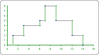
To create the waterfall chart using Error bars, do the following:

   1.   Add two columns with "X Errors" data and "Y Errors" data:

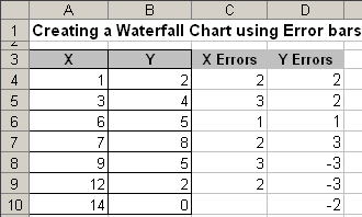
C4=A5-A4 and D4=B4, D5=B5-B4

   2.   Select the data range (in this example A4:B10).

   3.   Click the Chart Wizard button (or choose Insert -> Chart...).

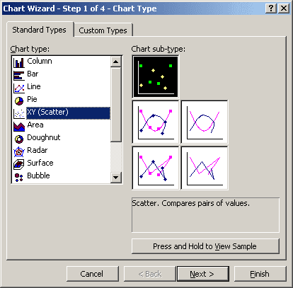
   4.   In the Chart Wizard dialog box, choose a XY (Scatter) type and the Scatter sub-type and then click Next >:

   5.   In the Step 2 of Chart Wizard, check the data and click Next >.

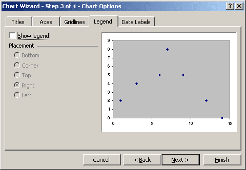
   6.   In the Step 3 of Chart Wizard:

• Remove Major gridlines on the Gridlines tab
• Remove the legend on the Legend tab.
  

   7.   In the Step 4 of Chart Wizard, click the Finish button.

   8.   In the popup menu choose Format Data Series....

In the Format Data Series dialog box:

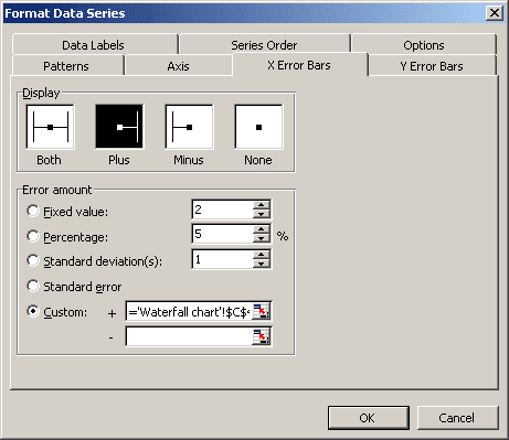
• On the X Error Bars tab:
  • In the Display group, select Plus
  • In the Error Amount group, select Custom: and in the + section select data range (in this example C4:C10).
  
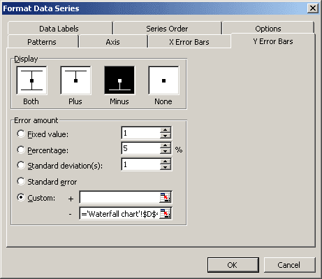
• On the Y Error Bars tab (see Adding error bars for more details about Error bars):
  • In the Display group, select Minus
  • In the Error Amount group, select Custom: and in the - section select data range (in this example D4:D10).
  

   6.   Right-click in one of the vertical Error bars and choose Format Y Error Bars... in the popup menu:

In the Format Error Bars dialog box, formal Y Error bars.

You can then make any other adjustments to get the look you desire.