How to freeze columns and rows

To freeze row or column headings (or both), follow these steps:

   1.   Click the cell to the right of the row labels and/or below any column labels you want to freeze. This highlights the cell.

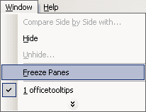
   2.   Select the Window menu, and then select Freeze Panes.

You might want to experiment on a large worksheet. Freeze the column and row headings, and then use the keyboard or the mouse to move around in the worksheet. As you do, the row and/or column headings remain locked in their positions. This enables you to view data in other parts of the worksheet without losing track of what that data represents.

When you have finished working with the frozen column and row headings, you can easily unfreeze them. Select the Window menu again and select Unfreeze Panes.