Creating a glossy thermometer chart

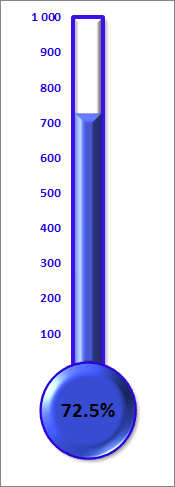
The trick involves creating a chart that uses a single cell (which holds a percentage value) as a data series.

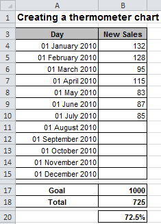
For example, a worksheet set up to track monthly progress toward a goal: 1,000 new sales in a year period. Cell B17 contains the goal value, and cell B18 contains a simple sum formula:

= SUM (B4:B15)

Cell B20 contains a formula that calculates the percent of goal:

= B18 / B17

As you enter new data in column B, the formulas display the current results.

To create the chart like this one, do the following:

   1.   Select cell B20 if you want to create a percentage axis or select cell B18 if you want to create a volume axis (in this example, used B18).

   2.   On the Insert tab, in the Charts group, choose the Column button:

Choose Clustered Column.

   3.   Remove the (x) axis and the legend.

   4.   To make the column occupy the entire width of the plot area, double-click the column to display the Format Data Point dialog box (or choose it in the popup menu). Then in the Series Options tab, change the Gap Width setting:

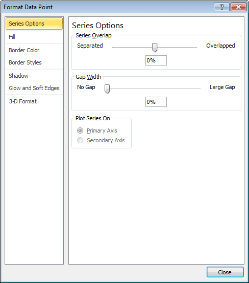
Set the Gap width to 0.

   5.   In the popup menu of axis choose Format Axis...:

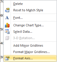
In the Format Axis dialog box, in the Axis Options tab, set the Minimum to 0 and the Maximum to 1 (if you use an percentage axis) or to 1000 (for this example):

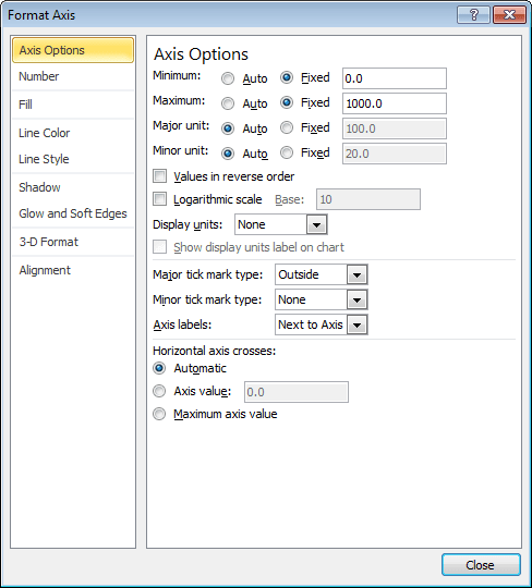
You can also hide the zero point in the axis (see How to hide points on the chart axis) and the axis line.

   6.   On the Insert tab, in the Illustrations group, select Shapes:

   7.   On the Shapes list, in the Basic Shapes group, choose Oval:

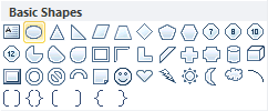
   8.   Format the shape and insert the data label (see How to insert cell content to the shape).

You can then make any other adjustments to get the look you desire.