Competition chart with residual data

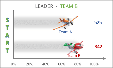
The trick of this chart is to show the additionally calculated data from specific cells in the chart labels.

To create a chart like the one above, do the following:

Add a new data

   1.   Create data for the chart:

• For the residual data (in this example, cells C14:D14),
• For the data series on the chart (in this example, cells C16:D17):

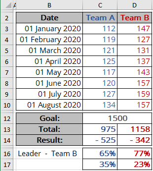
Cell B16 contains the formula to display a leader in the chart title. See how to display dynamically updated data in the chart title.

Create a chart

   2.   Select all necessary data - in this example, C2:D2, C16:D17.

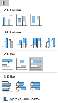
   3.   On the Insert tab, in the Charts group, click the Insert Column or Bar Chart button:

From the Insert Column or Bar Chart dropdown list, select 100% Stacked Bar:

Display the residual data

   4.   Select the second data series (the residual values), then do one of the following:

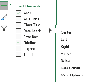
• Click on the Chart Elements button, select the Data Labels list, then select the position of the labels (the options depend on the data series chart type):
  
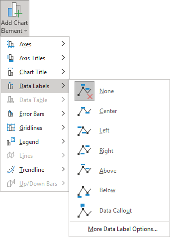
• On the Chart Design tab, in the Chart Layouts group, click the Add Chart Element button:
  

  From the Add Chart Element dropdown list, choose Data Labels, then select the place for the labels (the options depend on the data series chart type):

  
• Right-click on the second data series (residual data), then select Add Data Labels -> Add Data Labels in the popup menu:
  

Format data labels

   5.   Right-click on the data labels and select Format Data Labels... in the popup menu:

On the Format Data Labels pane, on the Label Options section, in the Label Contains group, check the Value From Cells option and then choose cells in the Data Label Range dialog box:

Optionally, hide the second data series

   6.   Right-click on the second data series (the residual values) and choose Format Data Series... in the popup menu:

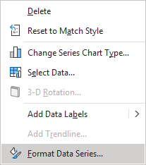
To make this data series invisible, on the Format Data Series pane, on the Series Options tab, in the Fill & Line group:

• In the Fill section, select No fill,
• In the Border section, select No line:

Make any other adjustments to get the look you desire.

See more:

• How to create dependent on a volume chart title.
• Creating a chart with dynamic labels.

See also this tip in French: Créer un graphique de concurrence avec des données résiduelles.